Probability And Bayesian Inference

When in doubt, Bayes it out

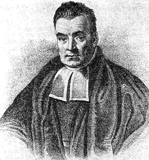
Everyone who has dipped their toes into Machine Learning or Statistics related fields has/will probably stumbled into This (In)famous Guy and His Rule:

Bayes Rule (with different letters than you might’ve seen):

$$\Large P(w|D) = \frac{P(D|w)P(w)}{P(D)}$$

where:

• $w$ denotes model parameters
• $D$ denotes the observed data

In short, the above formulation of Bayes theorem gives us the posterior probability over models. For now we’ll maximize it to pick a single best model. This point-estimate shortcut is called MAP, and we’ll get there soon enough:

$$\Large P(w|D) \propto P(D|w) \cdot P(w)$$

in order to find “The Best Model That Fits The Data”. Okay, so that’s a whole lot of letters, and a whole lot of terms. Maybe lets take a step back and build on some fundamentals.

If there’s one thing to take away from this reading:

It’s the (fairly self evident) phrase “The Best Model That Fits The Data”

I understand the phrase “The Best Model That Fits The Data” feels almost like a truism.

“Like of course, yes, I am trying to make a model that do the data good. Why else would I be doing the model?”

Understanding the following is actually quite core to much of much of Machine / Deep Learning in subsequent topics. Grasping the core of ‘priors’, ‘likelihoods’, ‘posteriors’, ‘beliefs’ etc. is core to the motivations of many architectures in both Predictive and Generative Modelling. And also whilst the phrase feels easy to say and understand, deriving it is non-trivial.

Why Those Letters? Why do any of this?

In Statistics / Machine Learning, we generally have some collected data, and want to create a useful model out of it that can help us do inference on a variety of things, whether that be for extrapolating data out of our domain, predicting on unseen data within the domain, classifying into dogs and cats, etc etc.

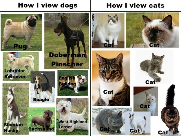
In most other readings, we would start with talking about “500 images of dogs and cats, labelling them 0s and 1s”. But its important to actually take a further step back and ask, why 0s and 1s in particular? And why ‘images of dogs and cats’?

Let us first explore the most fundamental perspective that will help us generalize better. Fundamentally, we begin from ‘Nature’, which is this magical abstraction that does everything in mysterious ways. In ‘Nature’, there is some incredibly complex, hidden mechanism that creates the data we observe. For this particular task, ‘Nature’ takes the form of the pixels of our image, and also the strange mechanism that composes a particular configuration of these pixels to form ‘cat imagery’. In other words, its not just particular set of pixels, but their complex and unexplainable relations to each other, that forms the image of a cat! We call this the ‘Underlying Data Generating Process’.

The Underlying Data Generating Process motivates us to denote the following:

$$\Large D = \left\{ (x_1, y_1), (x_2, y_2), ... (x_N, y_N) \right\}$$

where D is the set of cat and dog images $x$ and their labels $y$ that we actually collected, generated by this underlying process. N is just how many samples we gathered, a few hundred or thousand (not every possible image. The space of all possible 256 by 256 images is the unfathomably large part; our dataset $D$ is only a tiny, finite sample drawn from it.) According to the rules of The Universe, every single pair is independently sampled from some true, hidden joint distribution of nature that we want to model:

$$\Large (x_i, y_i) \sim P_{\text{true}}(x,y)$$

Ok, that’s fine and dandy. Where do I start fitting my model though?

Maximum (Log) Likelihood Estimation

As a recap as to what you may have learnt/heard in class, the likelihood function measures how well our hypothesis $H$, explains the evidence $E$. In this reading, $H$ is $w$ and $E$ is $D$. In other words, how well does our model $w$ explains the evidence $D$. In other words, a better model is one that explains the data better, which makes sense: If model $w_A$ gives a high probability to a high probability data point $(x_i, y_i)$, it is a better model than $w_b$ which gives a lower probability to that same data point. Here I’ll just write $d_i = (x_i, y_i)$. In (scuffed) notation,

$$\Large P(d_i | w_A) > P(d_i | w_B) \implies w_A \text{ explains } d_i \text{ better than } w_B$$

Since we have many data points we want to find a model that explains our entire dataset D. Again assuming independent sampling from the underlying data generation process, the total likelihood $\mathcal{L}(w ; D)$ of the dataset under a model $w$ is calculated by multiplying the individual probabilities of every single data point together:

$$\Large \mathcal{L}(w ; D) = P(d_1, d_2, \dots, d_N | w) = \prod_{i=1}^{N} P(d_i | w)$$

Just like before, if we have two competing models, the one that yields a higher total product is the superior model for our data:

$$\Large \mathcal{L}(w_A ; D) > \mathcal{L}(w_B ; D) \implies w_A \text{ explains the entire dataset better than } w_B$$

(Note: As you can imagine, with 256 by 256 pixels and 2 labels alone, each individual $d$ is of very small probability, so we’d rather apply a natural logarithm to turn things into additions:

$$\log \mathcal{L}(w ; D) = \log \left( \prod_{i=1}^{N} P(d_i | w) \right) = \sum_{i=1}^{N} \log P(d_i | w)$$

Also, note that yes, in this formulation of $P(D) = \prod_{i=1}^{N} P(d_i)$, it means the particular probability of our dataset D is very small. How come? Because we could have done data collection and gotten a very different result, since once again, our domain is so large for a 256 by 256 image with 2 labels! Even though the end product is still a bunch of cat and dog photos. Fortunately, this microscopic probability does not matter for MLE. Because our collected dataset $D$ is fixed and set in stone, $P(D)$ acts as a constant background property of ‘Nature’. Our only goal here is to change our model parameters $w$ to maximize the likelihood. You shouldn’t worry about the exact probability of prior of $D$, that is $P(D)$ itself; the core takeaway is to view our dataset as a finite proxy for the total domain. If our model learns to explain this representative sample exceptionally well, it will theoretically generalize to the entire domain of Nature just as well.)

TLDR: All this section is saying, is that the best fit of the data, is the model that maximizes likelihood of the data! Or the more common case, minimizes the negative log likelihood of the data (doing minimum and doing the log is more numerically stable.)

$$\Large w_{MLE} = \arg\max_{w} P(D|w)$$

(decomposed into each datapoint and with the log function:)

$$\Large w_{MLE} = \arg\max_{w} \sum_{i=1}^{N} \log P(d_i | w)$$

Great, all we do now is to find the MLE of our data?

Not quite. The MLE isn’t really Bayesian at all, since it never touches a prior over $w$ — it only asks “which single $w$ makes the data most likely?”. That makes it a point estimate: one best guess, rather than a full distribution describing how much we should believe in each possible $w$.

So what would the complete answer look like? The whole posterior, $P(w|D) = \frac{P(D|w)P(w)}{P(D)}$, prior and all. But look hard at that denominator: $P(D) = \int P(D|w)P(w)\,dw$ is an integral over every possible configuration of the weights. For anything bigger than a toy model it’s hopelessly intractable, and we genuinely cannot compute it. That single fact, the intractability of the evidence, is what quietly splits statistics into two camps, and it’s also what forces the convenient shortcut we’ll take later.

Frequentist? Bayesian? What is bro on about?

In your statistics class, you probably studied cases like “A coin is flipped $x$ times, here is the data, figure out the heads-to-tail odds for this possibly biased coin”. In other words, given our data, which we derive from some form of randomized sampling, we figure out some truth parameter $w$ that produced the data we observed. $w$ is fixed, constant, and immutable: sampling more data will never change what $w$ is, (unless we deform the coin to the point of no return and $w$ is somehow changed forever). If we simply sample more data, we can come to a correct conclusion about $w$, since what we observe will likely align with it!

• Frequentist: The underlying parameter $w$ is constant and true: it’s ridiculous to even suggest the notion of a probability distribution $P(w)$! Instead, we should define “Confidence Intervals” for our “Point Estimate”. Rather, it is the data $D$ that is the source of randomness, and with sufficient sampling, we can iron that out.
• Bayesian: In contrast to the above, the Bayesian treats $w$ as a random variable because a probability distribution over $w$ encodes our belief / uncertainty about it. The fixed, unchanging thing we condition on is the data $D$ we actually observed (it’s correct simply because it is what we collected). So $P(w)$ and $P(w|D)$ represent our state of knowledge about $w$ before and after seeing the data!

In other words, the Bayesian actually consider $P(w)$, a prior over over the model / parameters!

(If this whole frequentist-vs-Bayesian split is new to you, Jake VanderPlas’s Frequentism and Bayesianism: A Practical Introduction is the most readable take on it I know of.)

Big Brained Bayesians: The Posterior

(Joke title btw. Both perspectives have their place, but the Bayesian framing tends to earn its keep on really complex modelling tasks. The intuition is simple: the more expressive your model, whether that’s more parameters (deeper networks, higher-rank weight matrices), a larger domain of transformations it can represent, or higher-dimensional feature spaces, the more astronomically large the space of candidate weights becomes, and the overwhelming majority of those candidates are nonsense (random noise, overfitting artifacts, solutions that don’t generalize). A prior is exactly the tool that constrains that class of models down to the ones we’d find plausible before seeing a single data point. Will you consciously invoke “the perspective” in applied research? Probably not, but it quietly motivates many design choices, regularization, architecture, even the loss function, that constrain the model class and only feel obvious in hindsight.)

From earlier:

$$\Large P(w|D) = \frac{P(D|w)P(w)}{P(D)}$$

where the LHS is known as the Posterior: it’s the probability of the model $w$ given the observed data $D$ (probability of the hypothesis given the evidence). As you might imagine with the flipped conditioning, the semantics are also flipped compared to the Likelihood. Looking at the equation above, you could observe a relation:

$$\Large P(w|D) \propto P(D|w) \cdot P(w)$$

(once again, the Bayesian does not concern himself with the opinion or size of $P(D)$.) Here, your MLE (the likelihood term) fits right in, but now with an added $P(w)$ term. This prior acts as a regularization penalty; penalizing particular configurations of weights / parameters. If you choose a Gaussian prior centred around zero, you get L2 Regularization (Weight Decay). If you opt for the Laplace distribution, you get L1 Regularization (Lasso).

If you self-studied some ML concepts but never really got the reason behind the idea of ‘Regularization’, this is it! It’s not just a convenience for numerical stability (even though it does help). A choice of regularization influences the prior over the model class (a model class is the set of all possible functions that a specific architecture can form as you change its weights), which ensures that we aren’t just finding a solution that is a “good fit to the data”, but also a good fit to our priors.

Continuing from the MLE:

$$\large w_{MAP} = \arg\max_{w} P(w|D) = \arg\max_{w} \frac{P(D|w)P(w)}{P(D)} = \arg\max_{w} P(D|w) P(w)$$

The above is termed the Maximum A Posteriori (MAP) Estimation. MAP generalizes MLE by adding a prior: when that prior is uniform (uninformative), $P(w)$ is constant, drops straight out of the $\arg\max$, and MAP collapses right back into MLE. (note the $P(D)$ denominator plays no role in optimization since its always positive and does not depend on $w$. Once more, the Bayesian optimizer does not concern himself with the opinion or size of $P(D)$).

Okay cool. Can we get back to predicting cats and dogs?

Sure, just a few more equations to fully link everything together. Lets decompose the likelihood (no log) back to our $(x_i, y_i)$ tuple:

$$\Large P(D|w) = \prod_{i=1}^N P(d_i|w) = \prod_{i=1}^{N} P(x_i, y_i | w)$$

The following comes from the nature of our image and label: we define the semantic of ‘label over an image’, i.e the label $y$ is conditional on the image $x$. Decomposing:

$$\Large P(D|w) = \prod_{i=1}^{N} P(y_i | x_i; w) \cdot P(x_i)$$

(Note: Write $P(x_i)$ without $w$ because model weights have no control over how often cats walk in front of cameras in the real world. That part belongs purely to ‘Nature’, a.k.a the Cat Distribution System. The semicolon between $x_i$ and $w$ is crucial: It entails parameterization, i.e $y_i$ and $x_i$ are true random variables but the distribution is fixed due to the fixed nature of $w$. Yes, I know the Bayesian perspective will be eventually applied, but this equation exists in the MLE setting first. So just take it as ‘conditioning on a particular $w$ that is NOT a random variable’).

Now, let’s substitute this expanded joint likelihood back into Bayes’ Theorem to calculate the posterior distribution of our weights, $P(w|D)$, for, like, the third time this equation is shown:

$$\Large P(w|D) = \frac{P(D|w) \cdot P(w)}{P(D)}$$

If we expand the denominator $P(D)$ (the marginal likelihood or “evidence”) as the integral over all possible weight configurations, the equation becomes:

$$\Large P(w|D) = \frac{\left[ \prod_{i=1}^{N} P(y_i | x_i; w) \cdot P(x_i) \right] \cdot P(w)}{\int \left[ \prod_{i=1}^{N} P(y_i | x_i; w) \cdot P(x_i) \right] \cdot P(w) dw}$$

Note what the denominator decomposes into: It’s an integral because we are marginalizing across all possible $w$. The above assumes a continuous weight space (hence the integral): if it were discrete, the denominator would look something more like:

$$\Large P(D) = \sum_{\mathbf{w} \in \Omega} \left[ \prod_{i=1}^{N} P(y_i | x_i; \mathbf{w}) \cdot P(x_i) \right] \cdot P(\mathbf{w})$$

Because $\prod_{i=1}^{N} P(x_i)$ does not depend on the weights $w$, it behaves like a constant inside the denominator’s integral. This means we can pull it out of the integral (or summation):

$$\Large P(w|D) = \frac{\left( \prod_{i=1}^{N} P(x_i) \right) \cdot \left( \prod_{i=1}^{N} P(y_i | x_i; w) \right) \cdot P(w)}{\left( \prod_{i=1}^{N} P(x_i) \right) \cdot \int \left( \prod_{i=1}^{N} P(y_i | x_i; w) \right) \cdot P(w) dw}$$

which cancels out to:

$$\Large \frac{\left[ \prod_{i=1}^{N} P(y_i | x_i; w) \right] \cdot P(w)}{\int \left[ \prod_{i=1}^{N} P(y_i | x_i; w) \right] \cdot P(w) dw}$$

recalling the proportionality described earlier as part of the explanation of the Maximum A Posteriori:

$$\Large P(w|D) \propto \prod_{i=1}^{N} P(y_i | x_i; w) \cdot P(w)$$

(because the Bayesian optimizer does not concern himself with the denominator— you get it.) and there we have it! With regularization and maximizing the MLE (which necessitates maximizing likelihood / minimizing negative log likelihood, i.e our loss function of predicting cats as 1s and dogs as 0s), we can maximize the Maximum A Posteriori of our model, which gives us “the most likely model, given our data”!

Just one other note to wrap things up: choice of labels implies a probability distribution of our data. The choice of 1s as cat-ness was entirely our own design choice (a Bernoulli distribution). And here’s the punchline that ties the whole article together: if you model each $P(y_i|x_i;w)$ as a Bernoulli with the network outputting $\hat{y}_i$, then the negative log of that single term is exactly $-[y_i\log\hat{y}_i + (1-y_i)\log(1-\hat{y}_i)]$. Sum over the dataset and the MLE likelihood term we’ve spent this whole article maximizing is just Binary Cross-Entropy:

• $-\log \prod_{i=1}^{N} P(y_i|x_i;w) = - \sum_{i=1}^{N} \left[ y_i \log \hat{y}_i + (1 - y_i) \log(1 - \hat{y}_i) \right] = \text{BCE Loss}$

(This “negative log-likelihood = cross-entropy” identity is worked through carefully in Deep Learning by Goodfellow, Bengio & Courville, Ch. 5.)

Let’s Wrap it Up

Okay, let’s see what we covered so far:

The “Underlying Data Generating Process”: A neat little abstraction we use to motivate the idea of a dataset, and the probabilities associated thereof. This is itself a sort of vague phrase, but you can fit it to whatever context suits you: whether its a particular latent variable that generates the data (we will cover this later), or simply ‘some process’ we don’t care about, we just only want to learn the mapping between our $x$‘s and $y$‘s.

Maximum Likelihood Estimation (MLE): A core concept in ML that you should pretty much just replace in your head with the loss function. In that sense, our choice of labels + loss have the implicit effect of changing the landscape of the Maximum Likelihood: e.g choosing Focal Loss with a bunch of hyperparameter selections instead of plain Cross-Entropy causes a different probabilistic landscape to emerge. Or if you have some assumption about Gaussian-ness, MSE can be used. All this choice affects where the peak of our MLE lands.

Maximum A Posteriori (MAP): The Bayesian relative to MLE, this time with a neat little prior involved. We typically think of Regularization if our prior is over the model / weights $w$, but as you will observe later, it generalizes to anything that semantically resembles a Hypothesis: Say, with a latent variable.

Where do we go from here? Can we generalize further?

1. Generative Architectures, Variational Inference and VAEs

(This will start to dip into the literature / theory around Variational AutoEncoders + Variational Inference. You can go read the full other reading if its out!)

You’ve been hearing me throw the word “latent variable” around a bunch. This is because it neatly fits into something else we often think about in representation learning: The idea of compression and un-compression: from the observation space to the latent space, and vice versa. If you really think about it, the label of ‘cats’ and ‘dogs’ is a latent variable; it is a (learned) derivation of meaning from pixel / image space to some semantic space with one basis vector (cat-ness to dog-ness). Generalizing further, we could map from pixel space to some smaller but still high-dimensional vector space with various arbitrary semantic axis beyond just cats and dogs (what many modern day encoders do).

Denoting latent variables of $x_i$ and $z_i$, we can generalize beyond just the typical $y_i$ binary human label we created earlier:

$$\Large \left\{ (x_1, z_1), (x_2, z_2), ... (x_N, z_N) \right\}$$

and also define that $z_{i}$ generates $x_i$. In other words, some process exists:

$$x \sim p_\theta(x|z)$$

So now our $z$ is a learned latent that controls the generation of some output: like a chunky vector that is fed to a decoder and converted to a generated image. If your image is a fluffy Persian cat, $z$ adapts to represent “extreme fluffiness.” If it’s a hairless Sphinx cat, $z$ shifts to represent “zero fluffiness.”

How do we actually get a particular $z$? By learning an encoder that maps some input (usually some related image we want to generate) to the latent space! In the VAE literature, this gives us three major probabilistic pieces to learn and approximate:

• Prior $p_{\theta}(z)$
• Likelihood $p_{\theta}(x|z)$
• Approximate posterior $q_{\phi}(z|x)$ (note the $q$ and the $\phi$). The true posterior $p_\theta(z|x)$ is intractable (it hides that same nasty evidence integral), so the VAE learns an approximation $q_\phi$ to stand in for it. That swap is the entire reason VAEs exist.

Yes, we have to learn $z$, which is a “kind of parameter for generation” (it is a latent random variable which is distinct from the strict definition of a parameter, but convenient to think about it that way), in addition to parameters $\theta$ and $\phi$. Fun!

Once again, we are really getting quite out of scope, but as you might infer, many of the derivations for VAEs, and in general many Generative Architectures, have their roots in Bayesian inference. (The original Auto-Encoding Variational Bayes by Kingma & Welling is where the approximate-posterior trick was introduced.)

2. Diffusion models (something else generative too lol)

Without getting into too much detail, Diffusion models have “two processes”: a forward and backward trajectory. In the forward process, the image is systematically destroyed over $T$ steps by adding Gaussian noise at each step:

$$\Large q(x_t | x_{t-1}) = \mathcal{N}(x_t; \sqrt{1 - \beta_t}x_{t-1}, \beta_t \mathbf{I})$$

where $\beta_t$ is the noise schedule output at time $t$. In the reverse process, we convert from pure noise backwards to a clean image $x_0$. The reverse step is just remarkably Bayesian again — though there’s a catch. The true reverse $q(x_{t-1}|x_t)$ is intractable as written below (we don’t know the marginal $q(x_{t-1})$). What’s actually tractable, and what DDPMs use, is the reverse conditioned on the clean image, $q(x_{t-1}|x_t, x_0)$ — but the Bayesian skeleton is identical:

$$\Large q(x_{t-1} | x_t) = \frac{q(x_t | x_{t-1}) q(x_{t-1})}{q(x_t)}$$

there are many other nasties involving intractable Posteriors (for both this and the VAE case etc etc.), and a bunch of other optimizations that should be covered elsewhere, but hopefully you can see the pervasiveness of the framework. (The $x_0$-conditioned reverse posterior and the rest of the machinery are laid out in Denoising Diffusion Probabilistic Models by Ho, Jain & Abbeel.)